Tutorial 2 - Spatial Network analysis

Lesson objectives

This tutorial focuses on spatial networks and learn how to construct a routable directed graph for Networkx and find shortest paths along the given street network based on travel times or distance by car. In addition, we will learn how to calculate travel times matrices by public transport using r5py -library.

Tutorial

In this tutorial we will focus on a network analysis methods that relate to way-finding. Finding a shortest path from A to B using a specific street network is a very common spatial analytics problem that has many practical applications.

Python provides easy to use tools for conducting spatial network analysis. One of the easiest ways to start is to use a library called Networkx which is a Python module that provides a lot tools that can be used to analyze networks on various different ways. It also contains algorithms such as Dijkstra’s algorithm or A* algoritm that are commonly used to find shortest paths along transportation network.

Next, we will learn how to do spatial network analysis in practice.

Materials

In case you want to run the tutorial on your own computer, you can download this Notebook and related data from here:

• Download materials (93 MB)

• See Installation instructions to install the Python libraries needed for running this tutorial.

Typical workflow for routing

If you want to conduct network analysis (in any programming language) there are a few basic steps that typically needs to be done before you can start routing. These steps are:

1. Retrieve data (such as street network from OSM or Digiroad + possibly transit data if routing with PT).

2. Modify the network by adding/calculating edge weights (such as travel times based on speed limit and length of the road segment).

3. Build a routable graph for the routing tool that you are using (e.g. for NetworkX, igraph or OpenTripPlanner).

4. Conduct network analysis (such as shortest path analysis) with the routing tool of your choice.

1. Retrieve data

As a first step, we need to obtain data for routing. Pyrosm library makes it really easy to retrieve routable networks from OpenStreetMap (OSM) with different transport modes (walking, cycling and driving).

• Let’s first extract OSM data for Helsinki that are walkable. In pyrosm, we can use a function called osm.get_network() which retrieves data from OpenStreetMap. It is possible to specify what kind of roads should be retrieved from OSM with network_type -parameter (supports walking, cycling, driving).

from pyrosm import OSM, get_data
import geopandas as gpd
import pandas as pd
import networkx as nx

# We will use test data for Helsinki that comes with pyrosm
osm = OSM(get_data("helsinki_pbf"))

# Parse roads that can be driven by car
roads = osm.get_network(network_type="driving")
roads.plot(figsize=(10,10))

<AxesSubplot: >

roads

	access	area	bicycle	bridge	cycleway	foot	footway	highway	int_ref	lanes	...	surface	tunnel	width	id	timestamp	version	tags	osm_type	geometry	length
0	None	None	None	None	None	None	None	unclassified	None	2	...	paved	None	None	4236349	1380031970	21	{"name:fi":"Erottajankatu","name:sv":"Skillnad...	way	MULTILINESTRING ((24.94327 60.16651, 24.94337 ...	14.0
1	None	None	None	None	None	None	None	unclassified	None	2	...	paved	None	None	4243035	1543430213	12	{"name:fi":"Korkeavuorenkatu","name:sv":"H\u00...	way	MULTILINESTRING ((24.94567 60.16767, 24.94567 ...	51.0
2	None	None	None	None	None	None	None	residential	None	2	...	cobblestone	None	None	4243036	1543430213	21	{"hazmat:A":"destination","name:fi":"Fabianink...	way	MULTILINESTRING ((24.94944 60.16791, 24.94946 ...	86.0
3	None	None	None	None	None	None	None	unclassified	None	None	...	asphalt	None	None	4247500	1545207617	16	{"name:fi":"Yliopistonkatu","name:sv":"Univers...	way	MULTILINESTRING ((24.94540 60.16981, 24.94555 ...	14.0
4	None	None	None	None	None	None	None	secondary	None	2	...	cobblestone	None	None	4247501	1549629388	25	{"embedded_rails":"tram","name:fi":"Vilhonkatu...	way	MULTILINESTRING ((24.94745 60.17209, 24.94730 ...	13.0
...	...	...	...	...	...	...	...	...	...	...	...	...	...	...	...	...	...	...	...	...	...
1129	None	None	None	None	None	None	None	service	None	None	...	None	yes	None	675858710	1552243847	1	None	way	MULTILINESTRING ((24.94016 60.17018, 24.94017 ...	7.0
1130	None	None	None	None	None	None	None	service	None	None	...	None	None	None	675858712	1552243847	1	None	way	MULTILINESTRING ((24.94016 60.17028, 24.94016 ...	11.0
1131	None	None	None	None	None	None	None	service	None	None	...	None	None	None	675858713	1552243847	1	None	way	MULTILINESTRING ((24.94009 60.17028, 24.94010 ...	11.0
1132	None	None	None	None	None	None	None	service	None	None	...	None	None	None	675858714	1552243847	1	None	way	MULTILINESTRING ((24.94013 60.16982, 24.94013 ...	14.0
1133	None	None	None	None	None	None	None	service	None	None	...	None	yes	None	675858715	1552243847	1	None	way	MULTILINESTRING ((24.94010 60.17018, 24.94013 ...	40.0

1134 rows × 30 columns

Okay, now we have drivable roads as a GeoDataFrame for the city center of Helsinki. If you look at the GeoDataFrame (scroll to the right), we can see that pyrosm has also calculated us the length of each road segment (presented in meters). The geometries are presented here as MultiLineString objects. From the map above we can see that the data also includes short pieces of roads that do not lead to anywhere (i.e. they are isolated). This is a typical issue when working with real-world data such as roads. Hence, at some point we need to take care of those in someway (remove them (typical solution), or connect them to other parts of the network).

In OSM, the information about the allowed direction of movement is stored in column oneway. Let’s take a look what kind of values we have in that column:

roads["oneway"].unique()

array(['yes', None, 'no'], dtype=object)

As we can see the unique values in that column are "yes", "no" or None. We can use this information to construct a directed graph for routing by car. For walking and cycling, you typically want create a bidirectional graph, because the travel is typically allowed in both directions at least in Finland. Notice, that the rules vary by country, e.g. in Copenhagen you have oneway rules also for bikes but typically each road have the possibility to travel both directions (you just need to change the side of the road if you want to make a U-turn). Column maxspeed contains information about the speed limit for given road:

roads["maxspeed"].unique()

array(['30', '40', None, '20', '10', '5', '50'], dtype=object)

As we can see, there are also None values in the data, meaning that the speed limit has not been tagged for some roads. This is typical, and often you need to fill the non existing speed limits yourself. This can be done by taking advantage of the road class that is always present in column highway:

roads["highway"].unique()

array(['unclassified', 'residential', 'secondary', 'service', 'tertiary',
       'primary', 'primary_link', 'cycleway', 'footway', 'tertiary_link',
       'pedestrian', 'trail', 'crossing'], dtype=object)

Based on these values, we can make assumptions that e.g. residential roads in Helsinki have a speed limit of 30 kmph. Hence, this information can be used to fill the missing values in maxspeed. As we can see, the current version of the pyrosm tool seem to have a bug because some non-drivable roads were also leaked to our network (e.g. footway, cycleway). If you notice these kind of issues with any of the libraries that you use, please notify the developers by raising an Issue in GitHub. This way, you can help improving the software. For this given problem, an issue has already been raised so you don’t need to do it again (it’s always good to check if a related issue exists in GitHub before adding a new one).

Okay, but how can we make a routable graph out of this data of ours? Let’s remind us about the basic elements of a graph that we went through in the lecture slides:

So to be able to create a graph we need to have nodes and edges. Now we have a GeoDataFrame of edges, but where are those nodes? Well they are not yet anywhere, but with pyrosm we can easily retrieve the nodes as well by specifying nodes=True, when parsing the streets:

# Parse nodes and edges
nodes, edges = osm.get_network(network_type="driving", nodes=True)

# Plot the data
ax = edges.plot(figsize=(10,10), color="gray", lw=1.0)
ax = nodes.plot(ax=ax, color="red", markersize=2)

# Zoom in to take a closer look
#ax.set_xlim([24.9375, 24.945])
ax.set_ylim([60.17, 60.173])

(60.17, 60.173)

edges.head()

	access	area	bicycle	bridge	cycleway	foot	footway	highway	int_ref	lanes	...	width	id	timestamp	version	tags	osm_type	geometry	u	v	length
0	None	None	None	None	None	None	None	unclassified	None	2	...	None	4236349	1380031970	21	{"name:fi":"Erottajankatu","name:sv":"Skillnad...	way	LINESTRING (24.94327 60.16651, 24.94337 60.16644)	1372477605	292727220	9.370
1	None	None	None	None	None	None	None	unclassified	None	2	...	None	4236349	1380031970	21	{"name:fi":"Erottajankatu","name:sv":"Skillnad...	way	LINESTRING (24.94337 60.16644, 24.94340 60.16641)	292727220	2394117042	4.499
2	None	None	None	None	None	None	None	unclassified	None	2	...	None	4243035	1543430213	12	{"name:fi":"Korkeavuorenkatu","name:sv":"H\u00...	way	LINESTRING (24.94567 60.16767, 24.94567 60.16763)	296250563	2049084195	4.174
3	None	None	None	None	None	None	None	unclassified	None	2	...	None	4243035	1543430213	12	{"name:fi":"Korkeavuorenkatu","name:sv":"H\u00...	way	LINESTRING (24.94567 60.16763, 24.94569 60.16744)	2049084195	60072359	21.692
4	None	None	None	None	None	None	None	unclassified	None	2	...	None	4243035	1543430213	12	{"name:fi":"Korkeavuorenkatu","name:sv":"H\u00...	way	LINESTRING (24.94569 60.16744, 24.94571 60.16726)	60072359	6100704327	19.083

5 rows × 32 columns

Okay, as we can see now we have both the roads (i.e. edges) and the nodes that connect the street elements together (in red) that are typically intersections. However, we can see that many of the nodes are in locations that are clearly not intersections. This is intented behavior to ensure that we have full connectivity in our network. We can at later stage clean and simplify this network by merging all roads that belong to the same link (i.e. street elements that are between two intersections) which also reduces the size of the network.

Note

In OSM, the street topology is typically not directly suitable for graph traversal due to missing nodes at intersections which means that the roads are not splitted at those locations. The consequence of this, is that it is not possible to make a turn if there is no intersection present in the data structure. Hence, pyrosm will separate all road segments/geometries into individual rows in the data.

Let’s take a look what our nodes data look like:

nodes.head()

	lon	lat	tags	timestamp	version	changeset	id	geometry
0	24.943271	60.166514	None	1390926206	2	0	1372477605	POINT (24.94327 60.16651)
1	24.943365	60.166444	{'highway': 'crossing', 'crossing': 'traffic_s...	1383915357	6	0	292727220	POINT (24.94337 60.16644)
2	24.943403	60.166408	None	1374595731	1	0	2394117042	POINT (24.94340 60.16641)
3	24.945668	60.167668	{'highway': 'crossing', 'crossing': 'uncontrol...	1290714658	5	0	296250563	POINT (24.94567 60.16767)
4	24.945671	60.167630	{'traffic_calming': 'divider'}	1354578076	1	0	2049084195	POINT (24.94567 60.16763)

As we can see, the nodes GeoDataFrame contains information about the coordinates of each node as well as a unique id for each node. These id values are used to determine the connectivity in our network. Hence, pyrosm has also added two columns to the edges GeoDataFrame that specify from and to ids for each edge. Column u contains information about the from-id and column v about the to-id accordingly:

# Check last four columns
edges.iloc[:5,-4:]

	geometry	u	v	length
0	LINESTRING (24.94327 60.16651, 24.94337 60.16644)	1372477605	292727220	9.370
1	LINESTRING (24.94337 60.16644, 24.94340 60.16641)	292727220	2394117042	4.499
2	LINESTRING (24.94567 60.16767, 24.94567 60.16763)	296250563	2049084195	4.174
3	LINESTRING (24.94567 60.16763, 24.94569 60.16744)	2049084195	60072359	21.692
4	LINESTRING (24.94569 60.16744, 24.94571 60.16726)	60072359	6100704327	19.083

We can see that the geometries are now stored as LineString instead of MultiLineString. At this point, we can fix the issue related to having some pedestrian roads in our network. We can do this by removing all edges from out GeoDataFrame that have highway value in 'cycleway', 'footway', 'pedestrian', 'trail', 'crossing':

edges = edges.loc[~edges["highway"].isin(['cycleway', 'footway', 'pedestrian', 'trail', 'crossing'])].copy()
edges.plot()

<AxesSubplot: >

Now we can see, that some of the isolated edges were removed from the data. The character ~ (tilde) in the command above is a negation operator that is handy if you want to e.g. remove some rows from your GeoDataFrame based on criteria such as we used here.

2. Modify the data

At this stage, we have the necessary components to build a routable graph (nodes and edges) based on distance. However, in real life the network distance is not the best cost metric to use, because the shortest path (based on distance) is not necessarily always the optimal route in terms of travel time. Time is typically the measure that people value more (plus it is easier to comprehend), so at this stage we want to add a new cost attribute to our edges GeoDataFrame that converts the metric distance information to travel time (in seconds) based on following formula:

• <distance-in-meters> / (<speed-limit-kmph> / 3.6)

Before we can do this calculation, we need to ensure that all rows in maxspeed column have information about the speed limit. Let’s check the value counts of the column and also include information about the NaN values with dropna parameter:

# Count values
edges["maxspeed"].value_counts(dropna=False)

30      1110
None     628
40       422
10        50
20        36
5         21
50         2
Name: maxspeed, dtype: int64

As we can see, the rows which do not contain information about the speed limit is the second largest group in our data. Hence, we need to apply a criteria to fill these gaps. We can do this based on following “rule of thumb” criteria in Finland (notice that these vary country by country):

Road class	Speed limit within urban region	Speed limit outside urban region
motorway	100	120
motorway_link	80	80
trunk	60	100
trunk_link	60	60
primary	50	80
primary_link	50	50
secondary	50	50
secondary_link	50	50
tertiary	50	60
tertiary_link	50	50
unclassified	50	80
unclassified_link	50	50
residential	50	80
living_street	20	NA
service	30	NA
other	50	80

For simplicity, we can consider that all the roads in Helsinki Region follows the within urban region speed limits, although this is not exactly true (the higher speed limits start somewhere at the outer parts of the city region). For making the speed limit values more robust / correct, you could use data about urban/rural classification which is available in Finland from Finnish Environment Institute. Let’s first convert our maxspeed values to integers using astype() method:

edges["maxspeed"] = edges["maxspeed"].astype(float).astype(pd.Int64Dtype())
edges["maxspeed"].unique()

<IntegerArray>
[30, 40, <NA>, 20, 10, 5, 50]
Length: 7, dtype: Int64

As we can see, now the maxspeed values are stored in integer format inside an IntegerArray, and the None values were converted into pandas.NA objects that are assigned with <NA>. Now we can create a function that returns a numeric value for different road classes based on the criteria in the table above:

def road_class_to_kmph(road_class):
    """
    Returns a speed limit value based on road class, 
    using typical Finnish speed limit values within urban regions.
    """
    if road_class == "motorway":
        return 100
    elif road_class == "motorway_link":
        return 80
    elif road_class in ["trunk", "trunk_link"]:
        return 60
    elif road_class == "service":
        return 30
    elif road_class == "living_street":
        return 20
    else:
        return 50

Now we can apply this function to all rows that do not have speed limit information:

mask = edges["maxspeed"].isnull()

mask

0       False
1       False
2       False
3       False
4       False
        ...  
2767     True
2768     True
2769     True
2770     True
2771     True
Name: maxspeed, Length: 2269, dtype: bool

# Separate rows with / without speed limit information 
mask = edges["maxspeed"].isnull()
edges_without_maxspeed = edges.loc[mask].copy()
edges_with_maxspeed = edges.loc[~mask].copy()

# Apply the function and update the maxspeed
edges_without_maxspeed["maxspeed"] = edges_without_maxspeed["highway"].apply(road_class_to_kmph)
edges_without_maxspeed.head(5).loc[:, ["maxspeed", "highway"]]

	maxspeed	highway
30	30	service
47	30	service
48	30	service
49	30	service
50	30	service

Okay, as we can see now the maxspeed value have been updated according our criteria, and e.g. the service road class have been given the speed limit 30 kmph. Now we can recreate the edges GeoDataFrame by combining the two frames:

edges = pd.concat([edges_with_maxspeed, edges_without_maxspeed])
#edges = edges_with_maxspeed.append(edges_without_maxspeed)
edges["maxspeed"].unique()

<IntegerArray>
[30, 40, 20, 10, 5, 50]
Length: 6, dtype: Int64

Great, now all of our edges have information about the speed limit. We can also visualize them:

# Convert the value into regular integer Series (the plotting requires having Series instead of IntegerArray) 
edges["maxspeed"] = edges["maxspeed"].astype(int)
ax = edges.plot(column="maxspeed", figsize=(10,10), legend=True)

Finally, we can calculate the travel time in seconds using the formula we saw earlier and add that as a new cost attribute for our network:

edges["travel_time_seconds"] = edges["length"] / (edges["maxspeed"]/3.6)
edges.iloc[0:10, -4:]

	u	v	length	travel_time_seconds
0	1372477605	292727220	9.370	1.12440
1	292727220	2394117042	4.499	0.53988
2	296250563	2049084195	4.174	0.50088
3	2049084195	60072359	21.692	2.60304
4	60072359	6100704327	19.083	2.28996
5	6100704327	296250223	6.027	0.72324
6	264015226	25345665	9.644	1.15728
7	25345665	296248024	7.016	0.84192
8	296248024	426911766	4.137	0.49644
9	426911766	60072364	21.132	2.53584

Excellent! Now our GeoDataFrame has all the information we need for creating a graph that can be used to conduct shortest path analysis based on length or travel time. Notice that here we assume that the cars can drive with the same speed as what the speed limit is. Considering the urban dynamics and traffic congestion, this assumption might not hold, but for simplicity, we assume so in this tutorial.

3. Build a directed graph with pyrosm

We can use pyrosm library (as well as OSMnx) to easily build a directed graph. Let’s see how we can create a routable NetworkX graph using pyrosm with one command:

G = osm.to_graph(nodes, edges, graph_type="networkx")
G

<networkx.classes.multidigraph.MultiDiGraph at 0x7f2771a4c1c0>

Now we have a similar routable graph, but pyrosm actually does some additional steps in the background. By default, pyrosm cleans all unconnected edges from the graph and only keeps edges that can be reached from every part of the network. In addition, pyrosm automatically modifies the graph attribute information in a way that they are compatible with OSMnx that provides many handy functionalities to work with graphs. Such as plotting an interactive map based on the graph:

import osmnx as ox 
ox.plot_graph_folium(G)

Make this Notebook Trusted to load map: File -> Trust Notebook

4. Routing with NetworkX

Now we have everything we need to start routing with NetworkX (based on driving distance or travel time). But first, let’s again go through some basics about routing.

Basic logic in routing

Most (if not all) routing algorithms work more or less in a similar manner. The basic steps for finding an optimal route from A to B, is to:

1. Find the nearest node for origin location * (+ get info about its node-id and distance between origin and node)

2. Find the nearest node for destination location * (+ get info about its node-id and distance between origin and node)

3. Use a routing algorithm to find the shortest path between A and B

4. Retrieve edge attributes for the given route(s) and summarize them (can be distance, time, CO2, or whatever)

* in more advanced implementations you might search for the closest edge

This same logic should be applied always when searching for an optimal route between a single origin to a single destination, or when calculating one-to-many -type of routing queries (producing e.g. travel time matrices).

Find the optimal route between two locations

Next, we will learn how to find the shortest path between two locations using Dijkstra’s algorithm.

First, let’s find the closest nodes for two locations that are located in the area. OSMnx provides a handly function for geocoding an address ox.geocode(). We can use that to retrieve the x and y coordinates of our origin and destination.

# OSM data is in WGS84 so typically we need to use lat/lon coordinates when searching for the closest node

# Origin
orig_address = "Simonkatu 3, Helsinki"
orig_y, orig_x = ox.geocode(orig_address)  # notice the coordinate order (y, x)!

# Destination
dest_address = "Unioninkatu 33, Helsinki"
dest_y, dest_x = ox.geocode(dest_address) 

print("Origin coords:", orig_x, orig_y)
print("Destination coords:", dest_x, dest_y)

Origin coords: 24.9360071 60.1696202
Destination coords: 24.95107282256198 60.172212099999996

Okay, now we have coordinates for our origin and destination.

Find the nearest nodes

Next, we need to find the closest nodes from the graph for both of our locations. For calculating the closest point we use ox.distance.nearest_nodes() -function and specify return_dist=True to get the distance in meters.

# 1. Find the closest nodes for origin and destination
orig_node_id, dist_to_orig = ox.distance.nearest_nodes(G, X=orig_x, Y=orig_y, return_dist=True)
dest_node_id, dist_to_dest = ox.distance.nearest_nodes(G, X=dest_x, Y=dest_y, return_dist=True)

print("Origin node-id:", orig_node_id, "and distance:", dist_to_orig, "meters.")
print("Destination node-id:", dest_node_id, "and distance:", dist_to_dest, "meters.")

Origin node-id: 659998487 and distance: 27.888258768172825 meters.
Destination node-id: 1012307791 and distance: 24.7466116739603 meters.

Now we are ready to start the actual routing with NetworkX.

Find the fastest route by distance / time

Now we can do the routing and find the shortest path between the origin and target locations by using the dijkstra_path() function of NetworkX. For getting only the cumulative cost of the trip, we can directly use a function dijkstra_path_length() that returns the travel time without the actual path.

With weight -parameter we can specify the attribute that we want to use as cost/impedance. We have now three possible weight attributes available: 'length' and 'travel_time_seconds'.

• Let’s first calculate the routes between locations by walking and cycling, and also retrieve the travel times

# Calculate the paths 
metric_path = nx.dijkstra_path(G, source=orig_node_id, target=dest_node_id, weight='length')
time_path = nx.dijkstra_path(G, source=orig_node_id, target=dest_node_id, weight='travel_time_seconds')

# Get also the actual travel times (summarize)
travel_length = nx.dijkstra_path_length(G, source=orig_node_id, target=dest_node_id, weight='length')
travel_time = nx.dijkstra_path_length(G, source=orig_node_id, target=dest_node_id, weight='travel_time_seconds')

metric_path == time_path

True

travel_length

1189.9919999999997

travel_time

128.53734

Okay, that was it! Let’s now see what we got as results by visualizing the results.

For visualization purposes, we can use a handy function again from OSMnx called ox.plot_graph_route() (for static) or ox.plot_route_folium() (for interactive plot).

• Let’s first make static maps

# Shortest path based on distance
fig, ax = ox.plot_graph_route(G, metric_path)

# Add the travel time as title
ax.set_xlabel("Shortest path distance {t: .1f} meters.".format(t=travel_length))

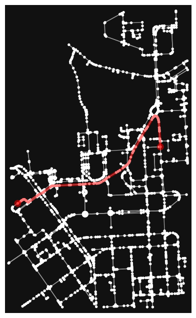
Text(0.5, 58.7222222222222, 'Shortest path distance  1190.0 meters.')

fig, ax = ox.plot_graph_route(G, time_path)

# Add the travel time as title
ax.set_xlabel("Travel time {t: .1f} minutes.".format(t=travel_time/60))

Text(0.5, 58.7222222222222, 'Travel time  2.1 minutes.')

Great! Now we have successfully found the optimal route between our origin and destination and we also have estimates about the travel time that it takes to travel between the locations by walking and cycling. As we can see, the route for both travel modes is exactly the same which is natural, as the only thing that changed here was the constant travel speed.

• Let’s still finally see an example how you can plot a nice interactive map out of our results with OSMnx:

ox.plot_route_folium(G, time_path, popup_attribute='travel_time_seconds')

Make this Notebook Trusted to load map: File -> Trust Notebook

Compute travel time matrices between multiple locations

When trying to understand the accessibility of a specific location, you typically want to look at travel times between multiple locations (one-to-many). Next, we will learn how to calculate travel time matrices using r5py Python library.

When calculating travel times with r5py, you typically need a couple of datasets:

• A road network dataset from OpenStreetMap (OSM) in Protocolbuffer Binary (.pbf) format:

  • This data is used for finding the fastest routes and calculating the travel times based on walking, cycling and driving. In addition, this data is used for walking/cycling legs between stops when routing with transit.

  • Hint: Sometimes you might need modify the OSM data beforehand, e.g., by cropping the data or adding special costs for travelling (e.g., for considering slope when cycling/walking). When doing this, you should follow the instructions on the Conveyal website. For adding customized costs for pedestrian and cycling analyses, see this repository.

• A transit schedule dataset in General Transit Feed Specification (GTFS.zip) format (optional):

  • This data contains all the necessary information for calculating travel times based on public transport, such as stops, routes, trips and the schedules when the vehicles are passing a specific stop. You can read about the GTFS standard here.

  • Hint: r5py can also combine multiple GTFS files, as sometimes you might have different GTFS feeds representing, e.g., the bus and metro connections.

Sample datasets

In the following tutorial, we use open source datasets from Helsinki Region:

• The point dataset for Helsinki has been obtained from Helsinki Region Environmental Services (HSY) licensed under a Creative Commons By Attribution 4.0.

• The street network for Helsinki is a cropped and filtered extract of OpenStreetMap (© OpenStreetMap contributors, ODbL license)

• The GTFS transport schedule dataset for Helsinki is an extract of Helsingin seudun liikenne’s (HSL) open dataset (Creative Commons BY 4.0).

Load the origin and destination data

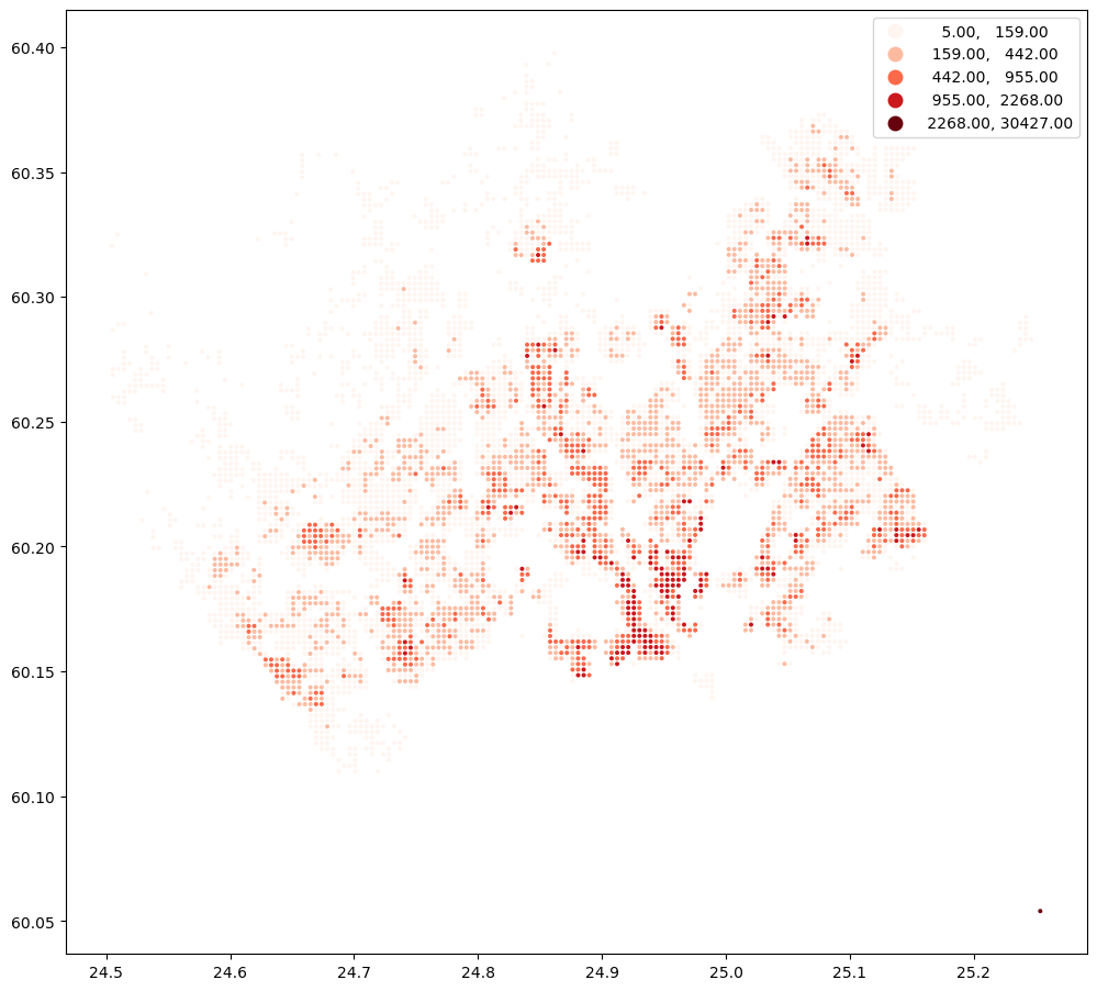
Let’s start by downloading a sample point dataset into a geopandas GeoDataFrame that we can use as our origin and destination locations. For the sake of this exercise, we have prepared a grid of points covering parts of Helsinki. The point data also contains the number of residents of each 250 meter cell:

import geopandas as gpd

# Calculate travel times to railway station from all grid cells
pop_grid_wfs = "https://kartta.hsy.fi/geoserver/wfs?request=GetFeature&typename=asuminen_ja_maankaytto:Vaestotietoruudukko_2021&outputformat=JSON"
pop_grid = gpd.read_file(pop_grid_wfs)

# Get centroids
points = pop_grid.copy()
points["geometry"] = points.centroid

# Reproject
points = points.to_crs(epsg=4326)
points.plot("asukkaita", scheme="natural_breaks", cmap="Reds", figsize=(12,12), legend=True, markersize=3.5)

<AxesSubplot: >

Next, we will geocode the address for Helsinki Railway station. For doing this, we can use oxmnx library and its handy .geocode() -function:

import osmnx as ox
from shapely.geometry import Point

# Find coordinates of the central railway station of Helsinki
lat, lon = ox.geocode("Rautatieasema, Helsinki")

# Create a GeoDataFrame out of the coordinates
station = gpd.GeoDataFrame({"geometry": [Point(lon, lat)], "name": "Helsinki Railway station", "id": [0]}, index=[0], crs="epsg:4326")
station.explore(max_zoom=13, color="red", marker_kwds={"radius": 12})

Make this Notebook Trusted to load map: File -> Trust Notebook

• Next, we will prepare the routable network

# Ignore some unnecessary warnings
import warnings
warnings.simplefilter('ignore')

%%time
import sys
# To increase the speed with local computer increase the amount of memory e.g. to 8 GB
sys.argv.append(["--max-memory", "5G"])

import datetime
from r5py import TransportNetwork, TravelTimeMatrixComputer, TransitMode, LegMode

# Filepath to OSM data
osm_fp = "data/Helsinki/Helsinki.osm.pbf"

transport_network = TransportNetwork(
    osm_fp,
    [
        "data/Helsinki/GTFS_Helsinki.zip"
    ]
)

WARNING: An illegal reflective access operation has occurred
WARNING: Illegal reflective access by org.mapdb.Volume$ByteBufferVol (file:/home/hentenka/.cache/r5py/r5-v6.6-all.jar) to method java.nio.DirectByteBuffer.cleaner()
WARNING: Please consider reporting this to the maintainers of org.mapdb.Volume$ByteBufferVol
WARNING: Use --illegal-access=warn to enable warnings of further illegal reflective access operations
WARNING: All illegal access operations will be denied in a future release

CPU times: user 6min 30s, sys: 5.25 s, total: 6min 36s
Wall time: 2min 8s

• After this step, we can do the routing

travel_time_matrix_computer = TravelTimeMatrixComputer(
    transport_network,
    origins=station,
    destinations=points,
    departure=datetime.datetime(2022,8,15,8,30),
    breakdown=True,
    transport_modes=[TransitMode.TRANSIT, LegMode.WALK],
)
travel_time_matrix = travel_time_matrix_computer.compute_travel_times()

Warning: SIGINT handler expected:libjvm.so+0xbe5900  found:python+0xd632a
Running in non-interactive shell, SIGINT handler is replaced by shell
Signal Handlers:
SIGSEGV: [libjvm.so+0xbe53b0], sa_mask[0]=11111111011111111101111111111110, sa_flags=SA_RESTART|SA_SIGINFO
SIGBUS: [libjvm.so+0xbe53b0], sa_mask[0]=11111111011111111101111111111110, sa_flags=SA_RESTART|SA_SIGINFO
SIGFPE: [libjvm.so+0xbe53b0], sa_mask[0]=11111111011111111101111111111110, sa_flags=SA_RESTART|SA_SIGINFO
SIGPIPE: [libjvm.so+0xbe53b0], sa_mask[0]=11111111011111111101111111111110, sa_flags=SA_RESTART|SA_SIGINFO
SIGXFSZ: [libjvm.so+0xbe53b0], sa_mask[0]=11111111011111111101111111111110, sa_flags=SA_RESTART|SA_SIGINFO
SIGILL: [libjvm.so+0xbe53b0], sa_mask[0]=11111111011111111101111111111110, sa_flags=SA_RESTART|SA_SIGINFO
SIGUSR2: [libjvm.so+0xbe5250], sa_mask[0]=00000000000000000000000000000000, sa_flags=SA_RESTART|SA_SIGINFO
SIGHUP: [libjvm.so+0xbe5900], sa_mask[0]=11111111011111111101111111111110, sa_flags=SA_RESTART|SA_SIGINFO
SIGINT: [python+0xd632a], sa_mask[0]=00000000000000000000000000000000, sa_flags=SA_ONSTACK
SIGTERM: [libjvm.so+0xbe5900], sa_mask[0]=11111111011111111101111111111110, sa_flags=SA_RESTART|SA_SIGINFO
SIGQUIT: [libjvm.so+0xbe5900], sa_mask[0]=11111111011111111101111111111110, sa_flags=SA_RESTART|SA_SIGINFO

travel_time_matrix.head()

	from_id	to_id	travel_time	routes	board_stops	alight_stops	ride_times	access_time	egress_time	transfer_time	wait_times	total_time	n_iterations
0	0	Vaestotietoruudukko_2021.1	86.0	[3002U, 2245A]	[1020502, 2611258]	[2611502, 2644205]	[25.0, 30.0]	3.0	9.5	16.0	[11.1, 3.0]	97.5	30.0
1	0	Vaestotietoruudukko_2021.2	97.0	[3002U, 2244]	[1020502, 2611258]	[2611502, 2643229]	[25.0, 30.0]	3.0	15.8	1.0	[5.1, 3.0]	82.8	9.0
2	0	Vaestotietoruudukko_2021.3	85.0	[3002E, 6243]	[1020502, 2611258]	[2611502, 2643206]	[25.0, 21.0]	3.0	26.0	1.0	[8.1, 3.0]	87.0	15.0
3	0	Vaestotietoruudukko_2021.4	84.0	[2213, 2244]	[1130111, 2611251]	[2611251, 2643215]	[37.0, 24.0]	10.5	16.4	0.0	[11.5, 16.0]	115.4	6.0
4	0	Vaestotietoruudukko_2021.5	72.0	[3002A, 7275, 6243]	[1020502, 2112261, 6170208]	[2111504, 6170209, 2643206]	[16.0, 22.0, 8.0]	3.0	1.7	4.9	[1.0, 7.7, 2.3]	66.7	1.0

• Now we can join the travel time information back to the population grid

geo = pop_grid.merge(travel_time_matrix, left_on="id", right_on="to_id")

geo.head()

	id	index	asukkaita	asvaljyys	ika0_9	ika10_19	ika20_29	ika30_39	ika40_49	ika50_59	...	routes	board_stops	alight_stops	ride_times	access_time	egress_time	transfer_time	wait_times	total_time	n_iterations
0	Vaestotietoruudukko_2021.1	688	5	50.60	99	99	99	99	99	99	...	[3002U, 2245A]	[1020502, 2611258]	[2611502, 2644205]	[25.0, 30.0]	3.0	9.5	16.0	[11.1, 3.0]	97.5	30.0
1	Vaestotietoruudukko_2021.2	703	7	36.71	99	99	99	99	99	99	...	[3002U, 2244]	[1020502, 2611258]	[2611502, 2643229]	[25.0, 30.0]	3.0	15.8	1.0	[5.1, 3.0]	82.8	9.0
2	Vaestotietoruudukko_2021.3	710	8	44.50	99	99	99	99	99	99	...	[3002E, 6243]	[1020502, 2611258]	[2611502, 2643206]	[25.0, 21.0]	3.0	26.0	1.0	[8.1, 3.0]	87.0	15.0
3	Vaestotietoruudukko_2021.4	711	7	64.14	99	99	99	99	99	99	...	[2213, 2244]	[1130111, 2611251]	[2611251, 2643215]	[37.0, 24.0]	10.5	16.4	0.0	[11.5, 16.0]	115.4	6.0
4	Vaestotietoruudukko_2021.5	715	11	41.09	99	99	99	99	99	99	...	[3002A, 7275, 6243]	[1020502, 2112261, 6170208]	[2111504, 6170209, 2643206]	[16.0, 22.0, 8.0]	3.0	1.7	4.9	[1.0, 7.7, 2.3]	66.7	1.0

5 rows × 27 columns

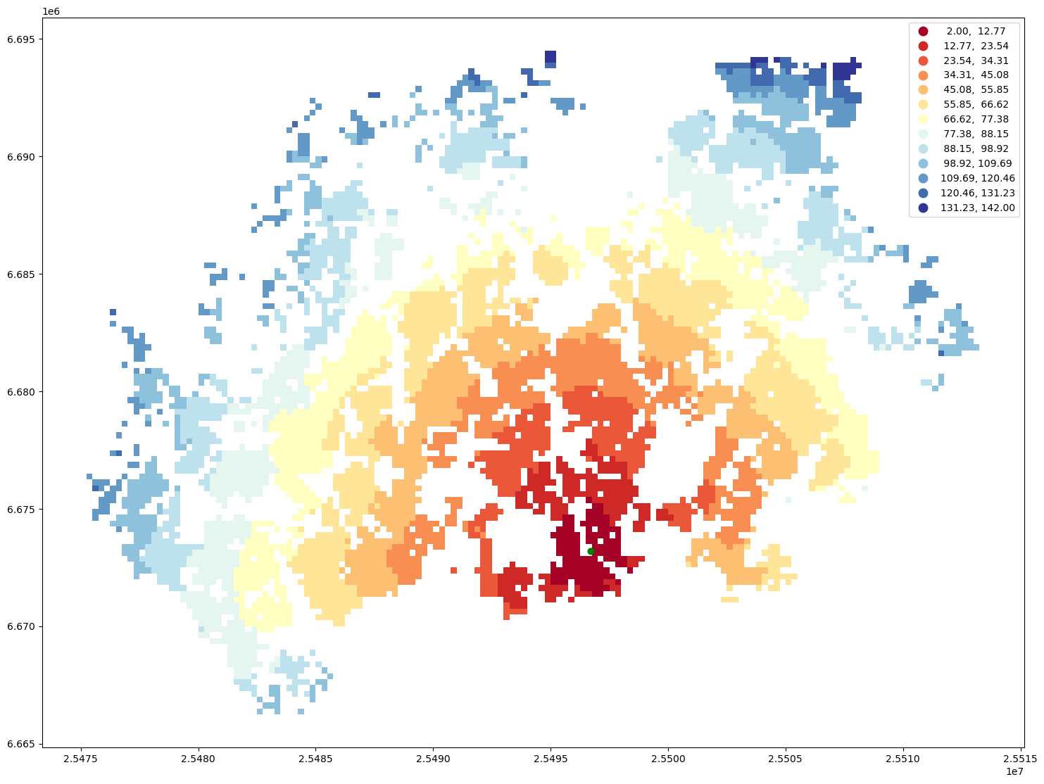
• Finally, we can visualize the travel time map and investigate how the railway station in Helsinki can be accessed from different parts of the region, by public transport.

import contextily as cx
ax = geo.plot(column="travel_time", cmap="RdYlBu", scheme="equal_interval", k=13, legend=True, figsize=(18,18))
ax = station.to_crs(crs=geo.crs).plot(ax=ax, color="green", markersize=40)
#cx.add_basemap(ax, crs=geo.crs, source=cx.providers.Stamen.Toner)

Calculate travel times by bike

In a very similar manner, we can calculate travel times by cycling. We only need to modify our TravelTimeMatrixComputer object a little bit. We specify the cycling speed by using the parameter speed_cycling and we change the transport_modes parameter to correspond to [LegMode.BICYCLE. This will initialize the object for cycling analyses:

tc_bike = TravelTimeMatrixComputer(
    transport_network,
    origins=station,
    destinations=points,
    speed_cycling=16,
    transport_modes=[LegMode.BICYCLE],
)
ttm_bike = tc_bike.compute_travel_times()

• Let’s again make a table join with the population grid

geo = pop_grid.merge(ttm_bike, left_on="id", right_on="to_id")

• And plot the data

ax = geo.plot(column="travel_time", cmap="RdYlBu", scheme="equal_interval", k=13, legend=True, figsize=(18,18))
ax = station.to_crs(crs=geo.crs).plot(ax=ax, color="green", markersize=40)
#cx.add_basemap(ax, crs=geo.crs, source=cx.providers.Stamen.Toner)

Calculate catchment areas

One quite typical accessibility analysis is to find out catchment areas for multiple locations, such as libraries. In the below, we will extract all libraries in Helsinki region and calculate travel times from all grid cells to the closest one. As a result, we have catchment areas for each library.

• Let’s start by parsing the libraries in Helsinki region, using pyrosm

from pyrosm import OSM, get_data

# Filepath to OSM data
osm_fp = "data/Helsinki/Helsinki.osm.pbf"

# Initialize the reader object
osm = OSM(osm_fp)

• Libraries can be parsed by using the get_pois -function, and passing a custom filter in which we specify that the amenity should be a library.

# Fetch libraries
libraries = osm.get_pois(custom_filter={"amenity": ["library"]})

• Some of the libraries might be in Polygon format, so we need to convert them into points by calculating their centroid:

# Convert the geometries to points
libraries["geometry"] = libraries.centroid
libraries.explore(color="red", marker_kwds={"radius": 6})

Make this Notebook Trusted to load map: File -> Trust Notebook

• Next, we can initialize our travel time matrix calculator using the libraries as the origins:

travel_time_matrix_computer = TravelTimeMatrixComputer(
    transport_network,
    origins=libraries,
    destinations=points,
    departure=datetime.datetime(2022,8,15,8,30),
    transport_modes=[TransitMode.TRANSIT, LegMode.WALK],
)
travel_time_matrix = travel_time_matrix_computer.compute_travel_times()

travel_time_matrix.shape

(567741, 3)

• As we can see, there are almost 57 thousand rows of data, which comes as a result of all connections between origins and destinations. Next, we want aggregate the data and keep only travel time information to the closest library:

# Find out the travel time to closest library
closest_library = travel_time_matrix.groupby("to_id")["travel_time"].min().reset_index()

closest_library

	to_id	travel_time
0	Vaestotietoruudukko_2021.1	50.0
1	Vaestotietoruudukko_2021.10	41.0
2	Vaestotietoruudukko_2021.100	60.0
3	Vaestotietoruudukko_2021.1000	43.0
4	Vaestotietoruudukko_2021.1001	47.0
...	...	...
5848	Vaestotietoruudukko_2021.995	21.0
5849	Vaestotietoruudukko_2021.996	18.0
5850	Vaestotietoruudukko_2021.997	21.0
5851	Vaestotietoruudukko_2021.998	53.0
5852	Vaestotietoruudukko_2021.999	48.0

5853 rows × 2 columns

Then we can make a table join with the grid in a similar manner as previously and visualize the data:

geo = pop_grid.merge(closest_library, left_on="id", right_on="to_id")

import contextily as cx
ax = geo.plot(column="travel_time", cmap="RdYlBu", scheme="natural_breaks", k=10, legend=True, figsize=(18,18))
ax = station.to_crs(crs=geo.crs).plot(ax=ax, color="green", markersize=40)
#cx.add_basemap(ax, crs=geo.crs, source=cx.providers.Stamen.Toner)

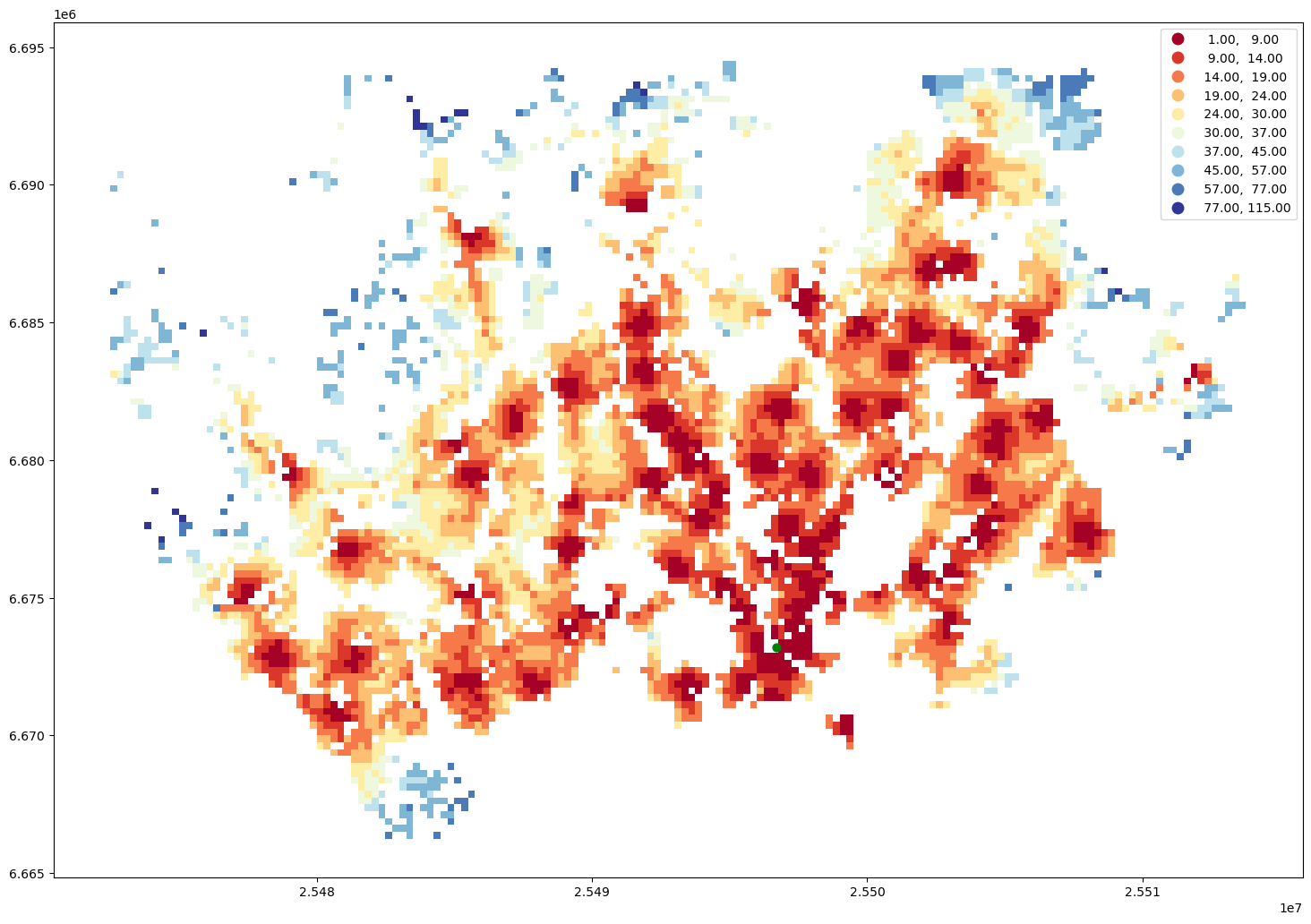
That’s it! As you can, see now we have a nice map showing the catchment areas for each library.

Analyze accessibility

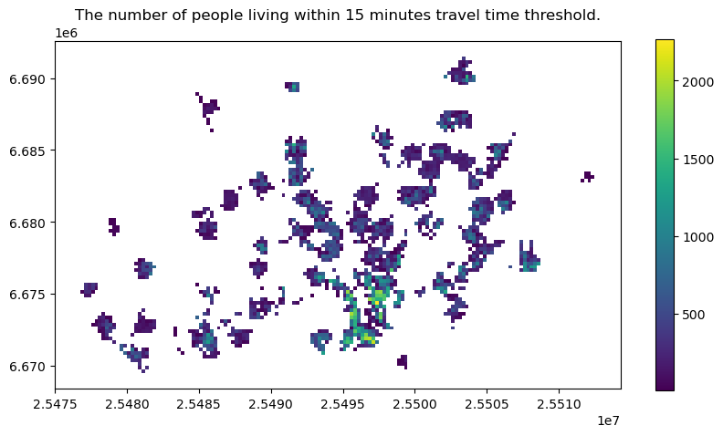
After we have calculated the travel times to the closest services, we can start analyzing accessibility. There are various ways to analyze how accessible services are. Here, for the sake of simplicity, we calculate the number of inhabitants that can reach the services within given travel time thershold (e.g. 15 minutes) by PT (or walking).

# Extract the grid cells within given travel time threshold
threshold = 15
access = geo.loc[geo["travel_time"]<=threshold].copy()

ax = access.plot(column="asukkaita", figsize=(10,5), legend=True)
ax.set_title(f"The number of people living within {threshold} minutes travel time threshold.");

Now we can easily calculate how many people or what is the proportion of people that can access the given service within the given travel time threshold:

pop_within_threshold = access["asukkaita"].sum()
pop_share = pop_within_threshold / geo["asukkaita"].sum()
print(f"Population within accessibility thresholds: {pop_within_threshold} ({pop_share*100:.0f} %)")

Population within accessibility thresholds: 627541 (52 %)

We can see that approximately 50 % of the population in the region can access a library within given time threshold. With this information we can start evaluating whether the level of access for the population in the region can be considered as “sufficient” or equitable. Naturally, with more detailed data, we could start evaluating whether e.g. certain population groups have lower access than on average in the region, which enables us to start studying the questions of justice and equity. Often the interesting question is to understand “who does not have access”? I.e. who is left out.

There are many important questions relating to equity of access that require careful consideration when doing these kind of analyses is for example what is seen as “reasonable” level of access. I.e. what should be specify as the travel time threshold in our analysis. Answering to these kind of questions is not straightforward as the accessibility thresholds (i.e. travel time budget) are very context dependent and normative (value based) by nature.

Cumulative opportunities

Another commonly used approach to analyze accessibility is to analyze how many services can a given individual (or group of individuals) access within given travel time budget. This is called cumulative opportunities measure.

# How many services can be reached from each grid cell within given travel time threshold?
travel_time_matrix.head()

	from_id	to_id	travel_time
0	33653057	Vaestotietoruudukko_2021.1	115.0
1	33653057	Vaestotietoruudukko_2021.2	NaN
2	33653057	Vaestotietoruudukko_2021.3	99.0
3	33653057	Vaestotietoruudukko_2021.4	94.0
4	33653057	Vaestotietoruudukko_2021.5	74.0

threshold = 15
# Count the number of opportunities from each grid cell
opportunities = travel_time_matrix.loc[travel_time_matrix["travel_time"]<=threshold].groupby("to_id")["from_id"].count().reset_index()

# Rename the column for more intuitive one
opportunities = opportunities.rename(columns={"from_id": "num_opportunities"})

# Merge with population grid
opportunities = pop_grid.merge(opportunities, left_on="id", right_on="to_id")

# Plot the results
ax = opportunities.plot(column="num_opportunities", figsize=(10,5), legend=True)
ax.set_title(f"Number of opportunities within {threshold} minutes."); 

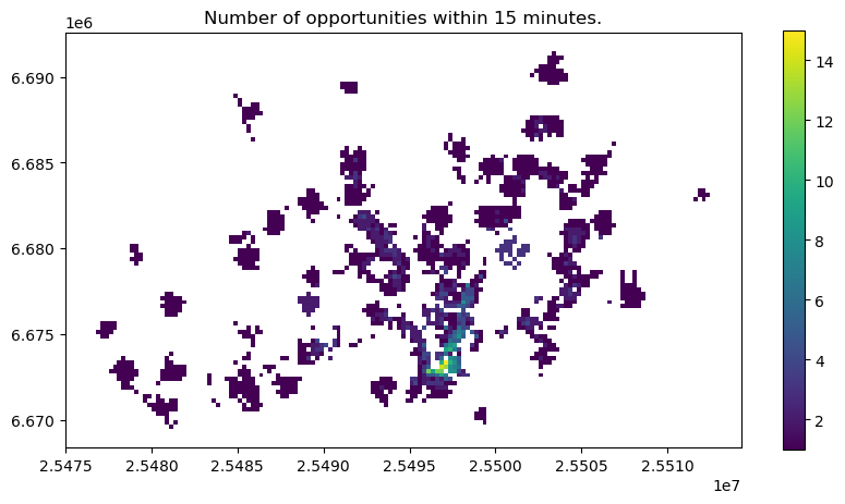
Now we can clearly see the areas with highest level of accessibility to given service. This is called cumulative opportunities measure or “Hansen’s Accessibility” measure after its developer.

At times one could still want apply a distance decay function to give more weight to the closer services and less to the services that are further away, and hence less likely to be visited by citizens who seek to use the service. This is called as time-weighted cumulative opportunities measure. There are also many other approaches to measure accessibility which are out of scope of this tutorial. In case you are interested in understanding more, I recommend reading following papers:

• Levinson, D. & H. Wu (2020). Towards a general theory of access.

• Wu, H. & D. Levinson (2020). Unifying access.