Tutorial I - Spatial analysis with Python

In this tutorial, we will take a quick tour to Python’s (spatial) data science ecosystem and see how we can use some of the fundamental open source Python packages, such as:

• pandas / geopandas

• shapely

• pysal

• pyproj

• osmnx

• matplotlib (visualization)

As you can see, we won’t use any GIS software for doing the programming (such as ArcGIS/arcpy or QGIS), but focus on learning the open source packages that are independent from any specific software. These libraries form nowadays not only the core for modern spatial data science, but they are also fundamental parts of commercial applications used and developed by many companies around the world.

Note

If you have experience working with the Python’s spatial data science stack, this tutorial probably does not bring much new to you, but to get everyone on the same page, we will all go through this introductory tutorial.

Contents

• Reading / writing spatial data

• Retrieving OpenStreetMap data

• Reprojections

• Spatial join

• Plotting data with matplotlib

Getting started

There are basically three options to run the codes in this tutorial:

1. Copy-Paste the codes from the website and run the codes line-by-line on your own computer with your preferred IDE (Jupyter Lab, Spyder, PyCharm etc.).

2. Download this Notebook (see below) and run it using Jupyter Lab which you should have installed by following the installation instructions.

3. Run the codes using Binder (see below) which is the easiest way, but has very limited computational resources (i.e. can be very slow).

Download the Notebook

You can download this tutorial Notebook to your own computer by clicking the Download button from the Menu on the top-right section of the website.

• Right-click the option that says .ipynb and choose “Save link as ..”

Run the codes on your own computer

Before you can run this Notebook, and/or do any programming, you need to launch the Jupyter Lab programming environment. The JupyterLab comes with the environment that you installed earlier (if you have not done this yet, follow the installation instructions). To run the JupyterLab:

1. Using terminal/command prompt, navigate to the folder where you have downloaded the Jupyter Notebook tutorial: $ cd /mydirectory/

2. Activate the programming environment: $ conda activate geo

3. Launch the JupyterLab: $ jupyter lab

After these steps, the JupyterLab interface should open, and you can start executing cells (see hints below at “Working with Jupyter Notebooks”).

Alternatively: Run codes in Binder (with limited resources)

Alternatively (not recommended due to limited computational resources), you can run this Notebook by launching a Binder instance. You can find buttons for activating the python environment at the top-right of this page which look like this:

Working with Jupyter Notebooks

Jupyter Notebooks are documents that can be used and run inside the JupyterLab programming environment containing the computer code and rich text elements (such as text, figures, tables and links).

A couple of hints:

• You can execute a cell by clicking a given cell that you want to run and pressing Shift + Enter (or by clicking the “Play” button on top)

• You can change the cell-type between Markdown (for writing text) and Code (for writing/executing code) from the dropdown menu above.

See further details and help for using Notebooks and JupyterLab from here.

Fundamental library: Geopandas

In this course, the most often used Python package that you will learn is geopandas. Geopandas makes it possible to work with geospatial data in Python in a relatively easy way. Geopandas combines the capabilities of the data analysis library pandas with other packages like shapely and fiona for managing spatial data. The main data structures in geopandas are GeoSeries and GeoDataFrame which extend the capabilities of Series and DataFrames from pandas. In case you wish to have additional help getting started with pandas, we recommend you to take a look at Chapter 3 from the openly available Introduction to Python for Geographic Data Analysis -book. The main difference between GeoDataFrames and pandas DataFrames is that a GeoDataFrame should contain (at least) one column for geometries. By default, the name of this column is 'geometry'. The geometry column is a GeoSeries which contains the geometries (points, lines, polygons, multipolygons etc.) as shapely objects.

Download the data

Before continuing this tutorial, download the data to your own computer and extract it to the same location where you have downloaded this notebook. Inside the ZIP file, there is a folder called data which is used in the following parts of the tutorial.

Reading and writing spatial data

Next we will learn some of the basic functionalities of geopandas. We have a couple of GeoJSON files stored in the data folder that we will use.

We can read the data easily with read_file() -function:

import geopandas as gpd

# Filepath
fp = "data/buildings.geojson"

# Read the file
data = gpd.read_file(fp)

# How does it look?
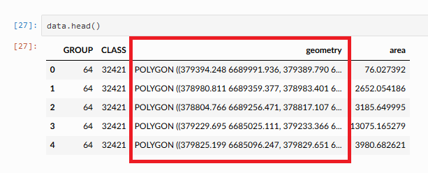
data.head()

	addr:city	addr:country	addr:housenumber	addr:housename	addr:postcode	addr:street	email	name	opening_hours	operator	...	start_date	wikipedia	id	timestamp	version	tags	osm_type	internet_access	changeset	geometry
0	Helsinki	None	29	None	00170	Unioninkatu	None	None	None	None	...	None	None	4253124	1542041335	4	None	way	None	NaN	POLYGON ((24.95121 60.16999, 24.95122 60.16988...
1	Helsinki	None	2	None	00100	Kaivokatu	ainfo@ateneum.fi	Ateneum	Tu, Fr 10:00-18:00; We-Th 10:00-20:00; Sa-Su 1...	None	...	1887	fi:Ateneumin taidemuseo	8033120	1544822447	27	{ "architect": "Theodor Höijer", "contact:webs...	way	None	NaN	POLYGON ((24.94477 60.16982, 24.9445 60.16981,...
2	Helsinki	FI	22-24	None	None	Mannerheimintie	None	Lasipalatsi	None	None	...	1936	fi:Lasipalatsi	8035238	1533831167	23	{ "name:fi": "Lasipalatsi", "name:sv": "Glaspa...	way	None	NaN	POLYGON ((24.93561 60.17045, 24.93555 60.17054...
3	Helsinki	None	2	None	00100	Mannerheiminaukio	None	Kiasma	Tu 10:00-17:00; We-Fr 10:00-20:30; Sa 10:00-18...	None	...	1998	fi:Kiasma (rakennus)	8042215	1553963033	30	{ "name:en": "Museum of Modern Art Kiasma", "n...	way	None	NaN	POLYGON ((24.93682 60.17152, 24.93662 60.1715,...
4	None	FI	None	None	None	None	None	None	None	None	...	None	None	15243643	1546289715	7	None	way	None	NaN	POLYGON ((24.93675 60.16779, 24.9366 60.16789,...

5 rows × 34 columns

As we can see, the GeoDataFrame contains various attributes in separate columns. The geometry column contains the spatial information. We can take a look of some of the basic information about our GeoDataFrame with command:

data.info()

<class 'geopandas.geodataframe.GeoDataFrame'>
RangeIndex: 486 entries, 0 to 485
Data columns (total 34 columns):
 #   Column              Non-Null Count  Dtype   
---  ------              --------------  -----   
 0   addr:city           86 non-null     object  
 1   addr:country        57 non-null     object  
 2   addr:housenumber    88 non-null     object  
 3   addr:housename      4 non-null      object  
 4   addr:postcode       54 non-null     object  
 5   addr:street         89 non-null     object  
 6   email               2 non-null      object  
 7   name                81 non-null     object  
 8   opening_hours       8 non-null      object  
 9   operator            7 non-null      object  
 10  phone               8 non-null      object  
 11  ref                 1 non-null      object  
 12  url                 8 non-null      object  
 13  website             20 non-null     object  
 14  building            486 non-null    object  
 15  amenity             26 non-null     object  
 16  building:levels     162 non-null    object  
 17  building:material   2 non-null      object  
 18  building:min_level  4 non-null      object  
 19  height              17 non-null     object  
 20  landuse             2 non-null      object  
 21  office              5 non-null      object  
 22  shop                5 non-null      object  
 23  source              3 non-null      object  
 24  start_date          87 non-null     object  
 25  wikipedia           47 non-null     object  
 26  id                  486 non-null    int32   
 27  timestamp           486 non-null    int32   
 28  version             486 non-null    int32   
 29  tags                181 non-null    object  
 30  osm_type            486 non-null    object  
 31  internet_access     1 non-null      object  
 32  changeset           66 non-null     float64 
 33  geometry            486 non-null    geometry
dtypes: float64(1), geometry(1), int32(3), object(29)
memory usage: 123.5+ KB

From here, we can see that our data is indeed a GeoDataFrame object with 486 entries and 34 columns. You can also get descriptive statistics of your data by calling:

data.describe()

	id	timestamp	version	changeset
count	4.860000e+02	4.860000e+02	486.000000	66.0
mean	1.400780e+08	1.455829e+09	4.849794	0.0
std	1.633527e+08	9.247528e+07	4.561162	0.0
min	8.253000e+03	1.197929e+09	1.000000	0.0
25%	2.294267e+07	1.374229e+09	2.000000	0.0
50%	1.228699e+08	1.493288e+09	3.000000	0.0
75%	1.359805e+08	1.530222e+09	7.000000	0.0
max	1.042029e+09	1.555840e+09	31.000000	0.0

In this case, we didn’t have many columns with numerical data, but typically you have numeric values in your dataset and this is a good way to get a quick view how the data look like.

Naturally, as the data is spatial, we want to visualize it to understand the nature of the data better. We can do this easily with plot() method:

data.plot()

<Axes: >

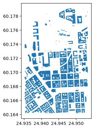
Now we can see that the data indeed represents buildings (in central Helsinki). Naturally we can also write this data to disk. Geopandas supports writing data to various data formats as well as to PostGIS which is the most widely used open source database for GIS. Let’s write the data as a Shapefile to the same data directory from where we read the data. When writing data to local disk you can use to_file() method:

# Output filepath
outfp = "data/buildings_copy.gpkg"
data.to_file(outfp)

Retrieving data from OpenStreetMap

Now we have seen how to read spatial data from disk. OpenStreetMap (OSM) is probably the most well known and widely used spatial dataset/database in the world. Also in this course, we will use OSM data frequently. Hence, let’s see how we can retrieve data from OSM using a library called omsnx. With osmnx you can easily download and extract data from anywhere in the world based on the Overpass API. You can use osmnx e.g. to retrieve OSM data around a given address and applying a 2 km buffer around this location. Hence, osmnx is a very flexible library in terms of specifying the area of interest.

OSM is a “database of the world”, hence it contains a lot of information about different things. With osmnx you can easily extract information about:

• street networks –> ox.graph_from_place(query) | ox.graph_from_polygon(polygon)

• buildings –> ox.features_from_place(query, tags={"buildings": True}) | ox.features_from_polygon(polygon, tags={"buildings": True})

• Amenities –> ox.features_from_place(query, tags={"amenity": True}) | ox.features_from_polygon(polygon, tags={"amenity": True})

• landuse –> ox.features_from_place(query, tags={"landuse": True}) | ox.features_from_polygon(polygon, tags={"landuse": True})

• natural elements –> ox.features_from_place(query, tags={"natural": True}) | ox.features_from_polygon(polygon, tags={"natural": True})

• boundaries –> ox.features_from_place(query, tags={"boundary": True}) | ox.features_from_polygon(polygon, tags={"boundary": True})

Let’s see how we can download and extract OSM data about buildings for Helsinki central area using osmnx:

import osmnx as ox
from shapely.geometry import box

# Bounding box for given area (Helsinki city centre)
bounds = [24.9351773, 60.1641551, 24.9534055, 60.1791068]

# Create a bounding box Polygon
bbox = box(*bounds)

# Retrieve buildings from the given area
buildings = ox.features_from_polygon(bbox, tags={"building": True})

buildings.head()

		geometry	addr:city	addr:country	addr:housenumber	addr:postcode	addr:street	air_conditioning	brand	building	contact:facebook	...	opening_hours:covid19	payment:cash	payment:mastercard	information	name:cs	type	last_roof_renovation	ele	electrified	nohousenumber
element	id
node	55211772	POINT (24.95158 60.17716)	Helsinki	FI	4	00530	John Stenbergin ranta	yes	Hilton Hotels & Resorts	yes	https://www.facebook.com/HiltonHelsinkiStrand/	...	NaN	NaN	NaN	NaN	NaN	NaN	NaN	NaN	NaN	NaN
	5643347516	POINT (24.94393 60.17412)	NaN	NaN	NaN	NaN	NaN	NaN	NaN	roof	NaN	...	NaN	NaN	NaN	NaN	NaN	NaN	NaN	NaN	NaN	NaN
relation	4198	POLYGON ((24.94898 60.17811, 24.94897 60.17826...	NaN	NaN	NaN	NaN	NaN	NaN	NaN	apartments	NaN	...	NaN	NaN	NaN	NaN	NaN	multipolygon	NaN	NaN	NaN	NaN
	5603	POLYGON ((24.93696 60.16574, 24.93791 60.16607...	NaN	NaN	NaN	NaN	NaN	NaN	NaN	yes	NaN	...	NaN	NaN	NaN	NaN	NaN	multipolygon	NaN	NaN	NaN	NaN
	5605	POLYGON ((24.93758 60.16662, 24.93788 60.16672...	NaN	NaN	NaN	NaN	NaN	NaN	NaN	apartments	NaN	...	NaN	NaN	NaN	NaN	NaN	multipolygon	NaN	NaN	NaN	NaN

5 rows × 148 columns

Let’s check how many buildings did we get:

len(buildings)

545

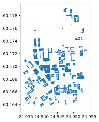
Okay, so in this sample there are over 500 buildings in the Helsinki city center area. Naturally, we would like to see them on a map. Let’s plot our data using plot() (might take some time as there are many objects to plot):

buildings.plot()

<Axes: >

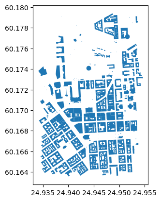
Great! As a result we got a map that seems to look correct.

Reprojecting data

As we can see from the previous maps that we have produced, the coordinates on the x and y axis hint that our geometries are represented in decimal degrees (WGS84). In many cases, you want to reproject your data to another CRS. Luckily, doing that is easy with geopandas. Let’s first take a look what the Coordinate Reference System (CRS) of our GeoDataFrame is. We can access the CRS information of the GeoDataFrame by accessing an attribute called crs:

buildings.crs

<Geographic 2D CRS: EPSG:4326>
Name: WGS 84
Axis Info [ellipsoidal]:
- Lat[north]: Geodetic latitude (degree)
- Lon[east]: Geodetic longitude (degree)
Area of Use:
- name: World.
- bounds: (-180.0, -90.0, 180.0, 90.0)
Datum: World Geodetic System 1984 ensemble
- Ellipsoid: WGS 84
- Prime Meridian: Greenwich

As a result, we get information about the CRS, and we can see that the data is indeed in WGS84. We can also see that the EPSG code for the CRS is 4326. We can easily reproject our data by using a method to_crs(). The easiest way to use the method is to specify the destination CRS as an EPSG code. Let’s reproject our data into EPSG 3067 which is the most widely used projected coordinate reference system used in Finland, EUREF-FIN:

projected = buildings.to_crs(epsg=3067)
projected.crs

<Projected CRS: EPSG:3067>
Name: ETRS89 / TM35FIN(E,N)
Axis Info [cartesian]:
- E[east]: Easting (metre)
- N[north]: Northing (metre)
Area of Use:
- name: Finland - onshore and offshore.
- bounds: (19.08, 58.84, 31.59, 70.09)
Coordinate Operation:
- name: TM35FIN
- method: Transverse Mercator
Datum: European Terrestrial Reference System 1989 ensemble
- Ellipsoid: GRS 1980
- Prime Meridian: Greenwich

As we can see, now we have an Projected CRS as a result. To confirm the difference, let’s take a look at the geometry of the first row in our original buildings GeoDataFrame and the projected GeoDataFrame. To select a specific row in data, we can use the iloc indexing:

orig_geom = buildings.iloc[4]["geometry"]
projected_geom = projected.iloc[4]["geometry"]

print("Orig:\n", orig_geom, "\n")
print("Proj:\n", projected_geom)

Orig:
 POLYGON ((24.9375782 60.1666195, 24.9378834 60.1667239, 24.9380204 60.1667708, 24.9383738 60.1665151, 24.938475 60.1664419, 24.9384826 60.1664364, 24.9384644 60.1664302, 24.9381689 60.166329, 24.937947 60.1662531, 24.9379354 60.1662615, 24.9376981 60.1664331, 24.9374847 60.1665875, 24.9375782 60.1666195), (24.9380198 60.1664339, 24.9380093 60.1664415, 24.9380613 60.1664593, 24.938074 60.1664501, 24.9381297 60.1664692, 24.9380864 60.1665005, 24.9380542 60.1664895, 24.9380219 60.1665128, 24.9380543 60.1665239, 24.9379768 60.16658, 24.9379475 60.1665699, 24.9378994 60.1666048, 24.9379289 60.1666149, 24.9378765 60.1666528, 24.9377978 60.1666259, 24.9378163 60.1666125, 24.9377221 60.1665803, 24.9379551 60.1664118, 24.9380198 60.1664339)) 

Proj:
 POLYGON ((385554.31899878354 6671754.572437016, 385571.61418283475 6671765.666812931, 385579.37784035725 6671770.650990822, 385598.0949883824 6671741.570552162, 385603.45498608454 6671733.24557284, 385603.8575069612 6671732.620069053, 385602.82623237354 6671731.961326439, 385586.08027316566 6671721.206265662, 385573.50548195647 6671713.140496254, 385572.89113039855 6671714.09580366, 385560.32264986954 6671733.611962159, 385549.020428861 6671751.171795174, 385554.31899878354 6671754.572437016), (385578.17306946206 6671733.143560318, 385577.6169656782 6671734.007893646, 385580.5637737497 6671735.899538935, 385581.2363684897 6671734.853259496, 385584.3929667008 6671736.883231213, 385582.09955670685 6671740.44301447, 385580.27488308103 6671739.274132089, 385578.56392962113 6671741.924184672, 385580.4000460868 6671743.103853063, 385576.295502162 6671749.483986066, 385574.6348493126 6671748.410282172, 385572.08767686307 6671752.379192268, 385573.7594245606 6671753.452548439, 385570.9841306813 6671757.762912904, 385566.5244039419 6671754.9044037545, 385567.50416222337 6671753.3804673795, 385562.166072896 6671749.958752856, 385574.5067199733 6671730.79518672, 385578.17306946206 6671733.143560318))

As we can see the coordinates that form our Polygon has changed from decimal degrees to meters. Let’s see what happens if we just call the geometries:

orig_geom

projected_geom

As you can see, we can draw the geometry directly in the screen, and we can easily see the difference in the shape of the two geometries. The orig_geom and projected_geom variables contain a Shapely geometry which is Polygon in this case. We can confirm this by checking the type:

type(orig_geom)

shapely.geometry.polygon.Polygon

These shapely geometries are used as the underlying data structure in most GIS packages in Python to present geometrical information. Shapely is fundamentally a Python wrapper for GEOS which is widely used library (written in C++) under the hood of many GIS softwares such as QGIS, GDAL, GRASS, PostGIS, Google Earth etc. Currently, there is ongoing work to vectorize all the GEOS functionalities for Python and bring those eventually into Shapely which will greatly boost the performance of all geometry related operations in Python ecosystem (approaching the same efficiency as PostGIS). Some of these improvements can already be found under the hood of latest version of geopandas.

Calculating area

One thing that is quite often interesting to know when working with spatial data, is the area of the geometries. In geopandas, we can easily calculate e.g. the area for each of our buildings by:

projected["building_area"] = projected.area
projected["building_area"].describe()

count     545.000000
mean     1032.930070
std      1120.966038
min         0.000000
25%       237.165839
50%       773.503344
75%      1396.511916
max      8419.604239
Name: building_area, dtype: float64

We calculated the area by calling area which is the attribute containing information about areas of the buildings measured based on the map units of the data. Hence, in this case because our data is projected in Euref-FIN the units that we stored in "building_area" column are square meters. It’s important to always keep in mind the CRS when calculating areas, distances etc. with geometries.

Spatial join

A commonly needed GIS functionality, is to be able to merge information between two layers using location as the key. Hence, it is somewhat similar approach as table join but because the operation is based on geometries, it is called spatial join. Next, we will see how we can conduct a spatial join and merge information between two layers. We will read all restaurants from the OSM for Helsinki Region, and combine information from restaurants to the underlying building (restaurants typically are within buildings). We will again use osmnx for reading the data, but this time we will get all amenities with tags “restaurant”, “bar” or “pub”:

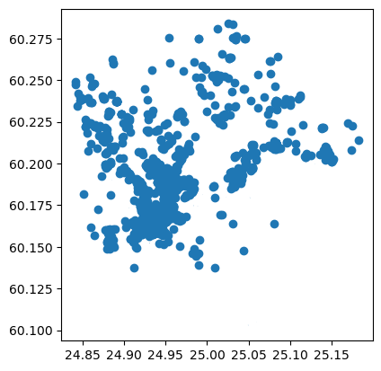
# Read restaurants
query = "Helsinki, Finland"
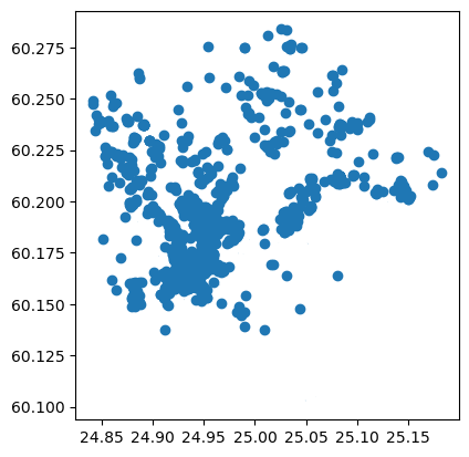
restaurants = ox.features_from_place(query, tags={"amenity": ["restaurant", "bar", "pub"]})
restaurants.plot()

<Axes: >

restaurants.info()

<class 'geopandas.geodataframe.GeoDataFrame'>
MultiIndex: 1621 entries, ('node', np.int64(25101780)) to ('way', np.int64(1276432323))
Columns: 242 entries, geometry to building:material
dtypes: geometry(1), object(241)
memory usage: 3.1+ MB

As we can see, the OSM for Helsinki contains more than 1500 restaurants altogether. As you can probably guess, the OSM data is far from “perfect” in terms of the quality of the restaurant listings. This is due to the voluntary nature of adding information to the OpenStreetMap, and the fact restaurants (as well as other POI features) are highly dynamic by nature, i.e. new amenities open and close all the time, and it is challenging to keep up to date with those changes (this is a challenge even for commercial companies).

Let’s also fetch buildings for the whole Helsinki area:

# Read restaurants
query = "Helsinki, Finland"
hki_buildings = ox.features_from_place(query, tags={"building": True})
hki_buildings.shape

(64097, 770)

hki_buildings.plot()

<Axes: >

There are altogether over 60 thousand buildings in Helsinki.

Joining data from buildings to the restaurants can be done easily using sjoin() function from geopandas:

# Join information from buildings to restaurants
join = gpd.sjoin(restaurants, hki_buildings)

# Print column names
print(join.columns)

# Show rows
join

Index(['geometry', 'addr:city_left', 'addr:country_left', 'amenity_left',
       'name_left', 'contact:website_left', 'cuisine_left',
       'opening_hours_left', 'diet:kosher_left', 'diet:vegan_left',
       ...
       'castle_type', 'old_name:en', 'payment:cheque',
       'payment:diners_club_right', 'payment:maestro', 'supervised',
       'service:vehicle:brakes', 'service:vehicle:oil_change',
       'service:vehicle:painting', 'service:vehicle:repairs'],
      dtype='object', length=1013)

		geometry	addr:city_left	addr:country_left	amenity_left	name_left	contact:website_left	cuisine_left	opening_hours_left	diet:kosher_left	diet:vegan_left	...	castle_type	old_name:en	payment:cheque	payment:diners_club_right	payment:maestro	supervised	service:vehicle:brakes	service:vehicle:oil_change	service:vehicle:painting	service:vehicle:repairs
element_left	id_left
node	25101780	POINT (24.85593 60.20729)	Helsinki	FI	pub	Muusan Krouvi	NaN	NaN	NaN	NaN	NaN	...	NaN	NaN	NaN	NaN	NaN	NaN	NaN	NaN	NaN	NaN
	25279508	POINT (24.86684 60.20897)	NaN	NaN	restaurant	Pikku Ranska	http://www.pikkuranska.com/	french	Mo-Th 10:30-22:15; Fr 11:00-23:00; Sa 12:00-23:00	NaN	NaN	...	NaN	NaN	NaN	NaN	NaN	NaN	NaN	NaN	NaN	NaN
	27392509	POINT (24.88337 60.18118)	NaN	NaN	restaurant	Ravintola Seurasaari	NaN	NaN	NaN	no	yes	...	NaN	NaN	NaN	NaN	NaN	NaN	NaN	NaN	NaN	NaN
	50808688	POINT (25.03395 60.2045)	Helsinki	NaN	pub	Foxy Bear	NaN	NaN	Mo-Th 10:00-22:00; Fr 10:00-23:00; Sa 11:00-23...	NaN	NaN	...	NaN	NaN	NaN	NaN	NaN	NaN	NaN	NaN	NaN	NaN
	50808951	POINT (25.03481 60.20454)	NaN	NaN	restaurant	Pikku-Hukka	NaN	scandinavian	Tu 11:00-15:00; We 11:00-20:00; Th,Fr 11:00-21...	NaN	NaN	...	NaN	NaN	NaN	NaN	NaN	NaN	NaN	NaN	NaN	NaN
...	...	...	...	...	...	...	...	...	...	...	...	...	...	...	...	...	...	...	...	...	...	...
way	1079281935	POLYGON ((25.05177 60.17933, 25.05189 60.17934...	Helsinki	NaN	restaurant	GlassRoom	NaN	NaN	NaN	NaN	NaN	...	NaN	NaN	NaN	NaN	NaN	NaN	NaN	NaN	NaN	NaN
	1079281940	POLYGON ((25.05153 60.17989, 25.05158 60.1798,...	Helsinki	NaN	restaurant	King Kebab	NaN	kebab	Mo-Sa 10:30-22:00; Su,PH 11:30-21:00	NaN	NaN	...	NaN	NaN	NaN	NaN	NaN	NaN	NaN	NaN	NaN	NaN
	1079281941	POLYGON ((25.05145 60.17971, 25.05161 60.17973...	Helsinki	NaN	restaurant	Fafa's	NaN	middle_eastern	Mo-Sa 10:30-22:00; PH,Su 12:00-20:00	NaN	NaN	...	NaN	NaN	NaN	NaN	NaN	NaN	NaN	NaN	NaN	NaN
	1093942712	POLYGON ((24.9699 60.19026, 24.96992 60.19026,...	NaN	NaN	restaurant	NaN	NaN	NaN	NaN	NaN	NaN	...	NaN	NaN	NaN	NaN	NaN	NaN	NaN	NaN	NaN	NaN
	1276432323	POLYGON ((25.04433 60.20683, 25.04453 60.20682...	Helsinki	FI	pub	Ravintola Siilinpesä	NaN	pizza	Mo-Tu 15:00-23:00; We-Th 15:00-00:00; Fr 12:00...	NaN	NaN	...	NaN	NaN	NaN	NaN	NaN	NaN	NaN	NaN	NaN	NaN

1624 rows × 1013 columns

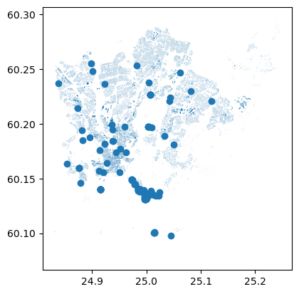
# Visualize the data as well
join.plot()

<Axes: >

As we can see from the above, now we have merged information from the buildings to restaurants. The geometries of the left GeoDataFrame, i.e. restaurants were kept by default as the geometries.

Selecting data using sjoin

One handy trick and efficient trick for spatial join is to use it for selecting data. We can e.g. select all buildings that intersect with restaurants by conducting the spatial join other way around, i.e. using the buildings as the left GeoDataFrame and the restaurants as the right GeoDataFrame:

# Merge information from restaurants to buildings (conducts selection at the same time)
join2 = gpd.sjoin(buildings, restaurants, how="inner", predicate="intersects")
join2.plot()

<Axes: >

As we can see (although the small building geometries are a bit poorly visible), the end result is a layer of buildings which intersected with the restaurants. This is a straightforward way to conduct simple spatial queries. You can specify with predicate parameter whether the binary predicate between the layers (i.e. the spatial relation between geometries) should be:

• intersects

• contains

• within

Plotting data with matplotlib

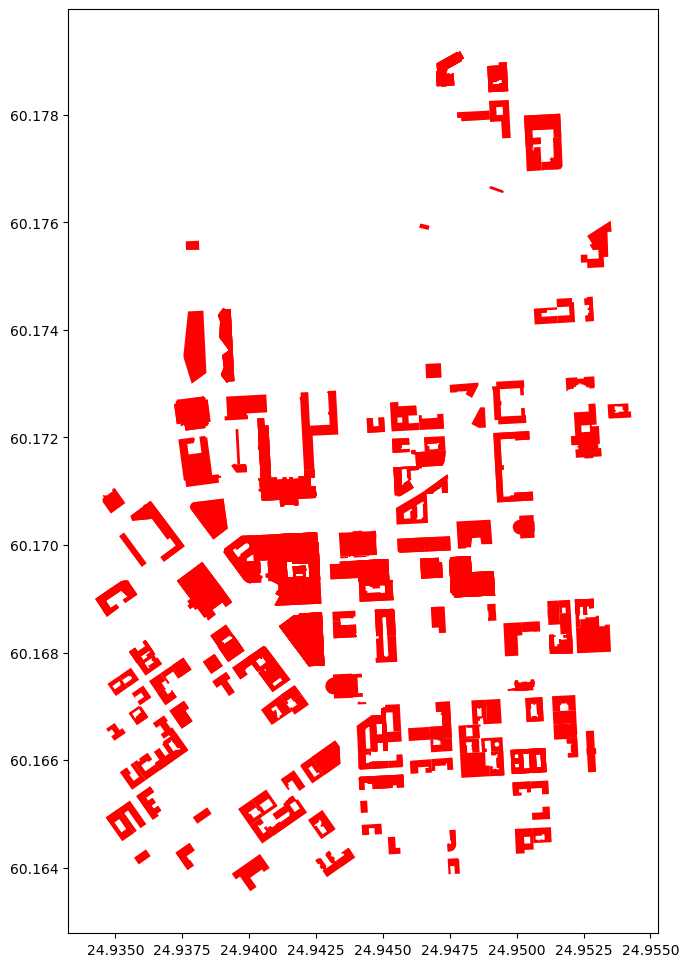
Thus far, we haven’t really made any effort to make our maps visually appealing. Let’s next see how we can adjust the appearance of our map, and how we can visualize many layers on top of each other. Let’s start by visualizing the buildings that we selected earlier and adjust a bit of the colors and figuresize. We can adjust the color of polygons with facecolor parameter and the figure size with figsize parameter that accepts a tuple of width and height as an argument:

ax = join2.plot(facecolor="red", figsize=(12,12))

join2.columns

Index(['geometry', 'addr:city_left', 'addr:country_left',
       'addr:housenumber_left', 'addr:postcode_left', 'addr:street_left',
       'air_conditioning_left', 'brand_left', 'building_left',
       'contact:facebook_left',
       ...
       'roof:levels_right', 'seamark:small_craft_facility:category',
       'seamark:type', 'building:colour_right', 'roof:shape_right',
       'building:part', 'height_right', 'roof:height_right', 'indoor',
       'building:material_right'],
      dtype='object', length=391)

Now with the bigger figure size, it is already a bit easier to see the selected buildings that have a restaurant inside them (according OSM). Let’s color our buildings based on the building type. Hence, each building type category will receive a different color:

ax = join2.plot(column="building_left", cmap="RdYlBu", figsize=(12,12), legend=True)

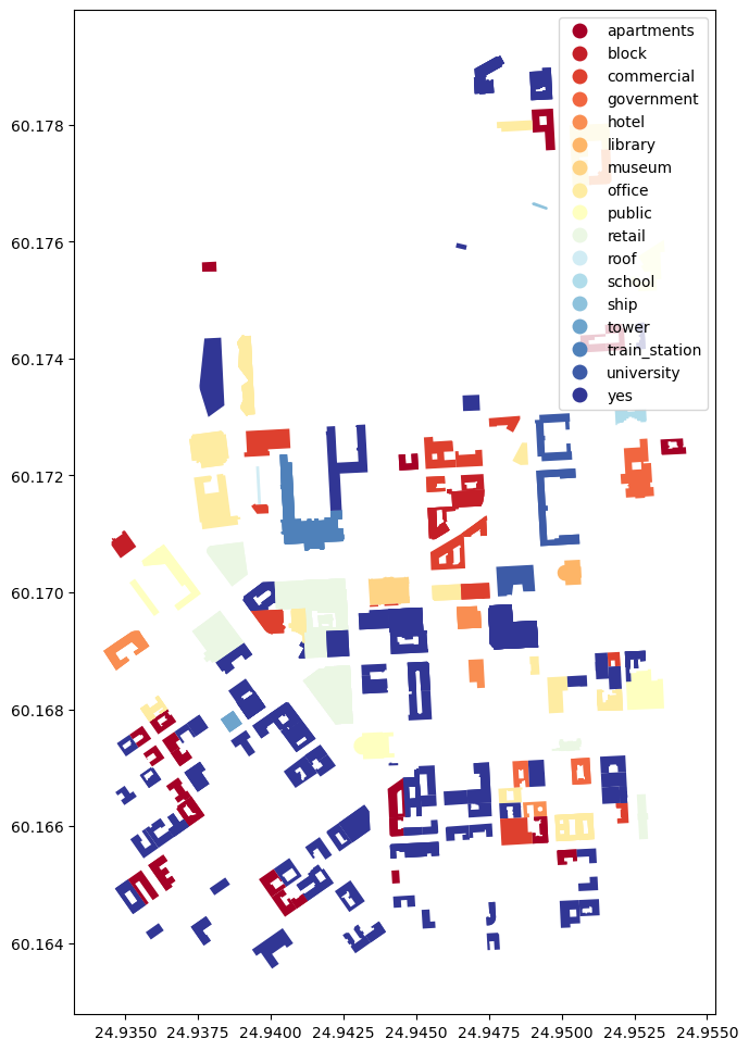
Now we used the parameter column to specify the attribute that is used to specify the color for each building (can be categorical or continuous). We used cmap to specify the colormap for the categories and we added the legend by specifying legend=True.

To get a bit more context to our visualizaton. Let’s also add roads with our buildings. To do that we first need to extract the roads from OSM:

# Get roads (retrieves walkable roads by default)
G = ox.graph_from_polygon(bbox)

# Parse roads from the graph
roads = ox.graph_to_gdfs(G, nodes=False, edges=True) 

Now we can continue and add the roads as a layer to our visualization with gray line color:

# Plot the map again
ax = join2.plot(column="building_left", cmap="RdYlBu", figsize=(12,12), legend=True)

# Plot the roads into the same axis
ax = roads.plot(ax=ax, edgecolor="gray", linewidth=0.75)

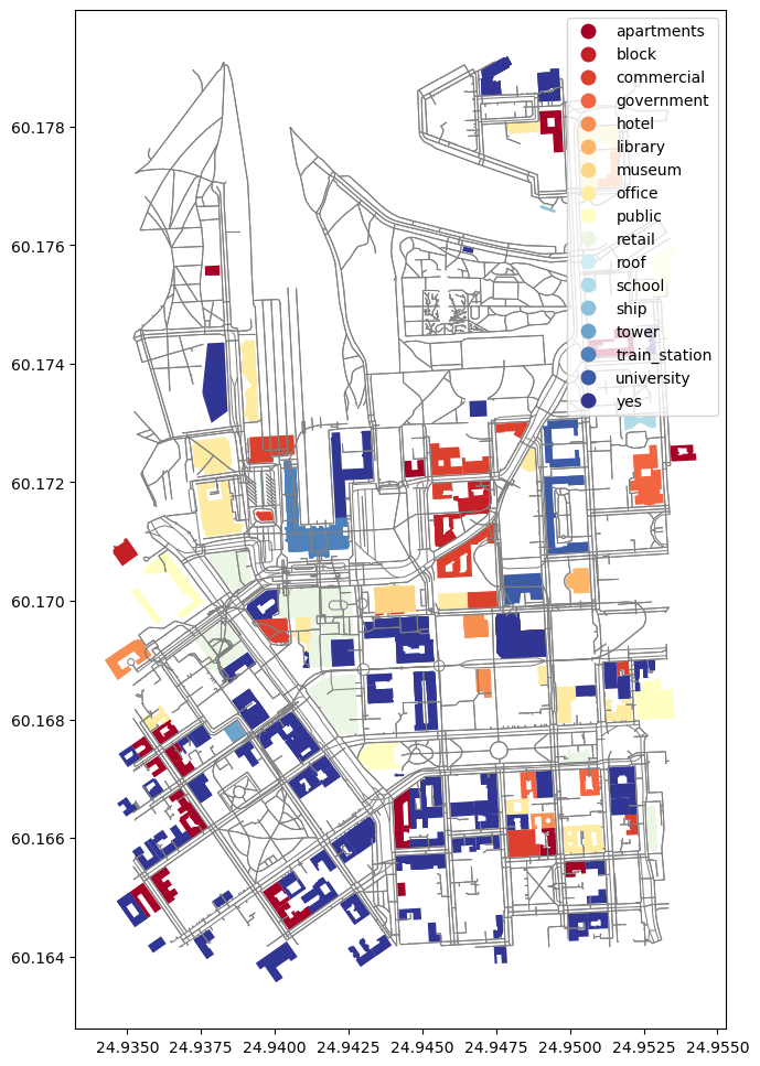
Perfect! Now it is much easier to understand our map because the roads brought much more context (assuming you know Helsinki). We ware able to add the roads to the same map by specifying the ax parameter to point to the axis that we received when first plotting the join2 (i.e. selected buildings). In a similar manner, you can add as many layers in your map as you wish. Let’s still do a small visual trick and specify that the background color in our map is black instead of white. This can be done easily by changing the style of matplotlib visualization renderer:

# Import matplotlib pyplot and use a dark_background theme
import matplotlib.pyplot as plt
plt.style.use("dark_background")

# Plot the map again
ax = join2.plot(column="building_left", cmap="RdYlBu", figsize=(12,12), legend=True)

# Plot the roads into the same axis
ax = roads.plot(ax=ax, edgecolor="gray", linewidth=0.75)

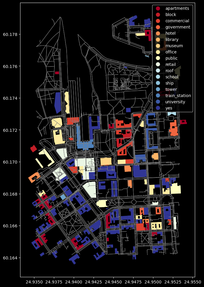
Awesome! Now we have a nice dark theme with our map. With this information you should be able to get going with Exercise 1.

Further information

For further information, we recommend reading the Chapter 6 from the Introduction to Python for Geographic Data Analysis -book.

We also recommend checking the materials from Automating GIS Processes -course (GIS things) and Geo-Python -course (intro to Python and data analysis with pandas). In addition, we always recommend to check the latest documentation from the websites of the libraries:

• geopandas

• osmnx

• matplotlib

• pandas